KDA Doesn't Care About the Future

Written: September 15, 2026

Product pitch

TorchTitan has been working on enabling new models. As you most likely know, most new models have moved away from purely global causal attention and now do some combo of GCA (global causal attention) + local attention. We call these hybrid models. They optionally mix in sparse attention for some or all of the layers that used to be GCA.

It is hard to be nimble in pytorch/pytorch - this is a good and a bad thing. We want to build out useful apis that enable researchers and implementers to get the most out of pytorch. Our Linear Attention apis have been severely lacking here. And our Sparse Apis have been decent through flex-attention but only when sparse granularity is largish (128,128)+. Soooo what are we to do!

Attention Gym is changing!

We are coalescing development of these fun new attention flavors here. We have built a number of primitives for gdn and kda and have been integrating them into torchtitan’s training and RL(inference) stack. As well we have been adding more sparse primitives to enable performant DSv4 training in Titan.

If you want to try the pieces together, here’s a full end-to-end KDA/GDN training example: a small single-device training loop with reference and fused backends, full-graph compilation, and profiling.

“But Driss why would I not just use FLA” That is a great question insightful reader! My honest answer: we pytorch developers are humans. We need a place to explore ideas, find common abstractions, figure out what works and what doesn’t. Attention gym is that place for me and others. Long term I would love to develop something as extensible as Flex Linear Attention but right now - I don’t see it. As well, AI has kind of thrown a wrench into this generalization thing we like doing.I have not given up! And as Dijkstra says: “The purpose of abstracting is not to be vague, but to create a new semantic level in which one can be absolutely precise.” If you want to have some influence on where we invest our time; use the repo, open issues and give us feedback. We are dogfooding in torchtitan but would love to hear from other voices.

Another more polished answer is that the components we are offering are more specialized to the latest hardware and this allows us to eke out nontrivial performance gains.These performance gains can be very large, but numbers are numbers, and I don’t want to include comparisons in this particular blog post. We have fully integrated CuDNN’s uber mega kernels, a robust CP implementation, paid special attention to making everything cuda-graphable. But if you are using FLA and it works for you and don’t want to switch I get it. It’s an awesome project and I personally have learned so much from it :)

Pitch done - TLDR

I was working on the intra-chunk kernels for Kimi Delta Attention(KDA) and found that there was a subtle implementation choice that has the potential to break causality. I used TorchTitan to test whether the model could learn to exploit it.

What is causality anyways

I think this phrase is a little too anthropomorphized. A better one is; training inference mismatch. That’s it. We call it causality because this particular form of mismatch is when you let a token at position $N$ receive information from token $M$ , for some $M > N$ . And in essence $N$ can see the future. This unsurprisingly really helps with the task of next token prediction. What are some ways this might happen;

you forget to invoke F.scaled_dot_product_attention(..., is_causal=True). That is an obvious one. There are some other more subtle forms;
Expert choice routing
Blockwise scaling of inputs during training

etc etc

This can be subtle, because during training there isn’t anything actually wrong with this. Either you have a massive information leak and you will see your loss decrease very very rapidly; or it will be a slow trickle. You might even think damn i really did something with this datamix!. Don’t be fooled, the problems only show up when you try to serve this model using auto-regressive token generation. The model learned that it’s only going to see batches of tokens and that this information from token $M$ will always be there to influence what it should predict at token $N$ . That’s what it learned during training, but at inference, token $M$ doesn’t exist yet. We’re building up the sequence one token at a time, and the result is you’ve trained this cracked model, but at inference time, it’s going to underperform relative to what you saw during training!

Training

Inference

Don’t just take my word for it

MatX’s “Future leakage in block-quantized attention” is a really really nice blog. The causal break it found has to do with low precision attention. When values share a quantization scale across token positions, a future outlier can increase that scale and make an earlier value underflow. Seems harmless but models are sneaky, trixy little hobbits and they use signals in remarkable ways!

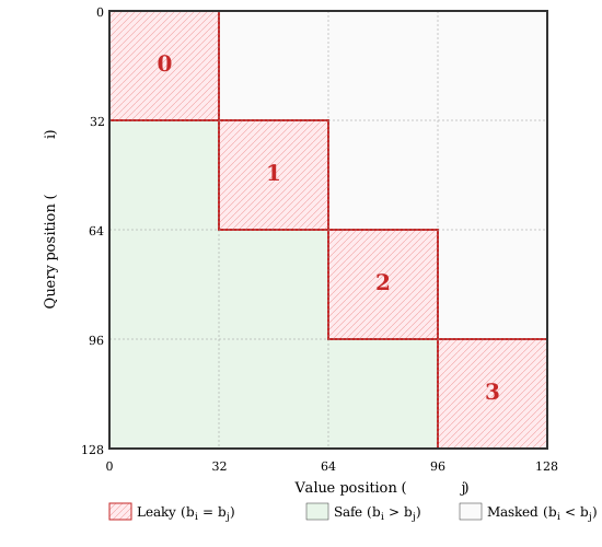
MatX's query-by-value matrix, divided into 32-token blocks. Red hatched diagonal blocks can leak future information through shared value quantization scales; green earlier blocks are safe from this leak, and gray later blocks are masked. — Figure from MatX, Future leakage in block-quantized attention

MX quantization shares one scale across 32 elements along the reduction dimension. In attention’s second GEMM, $P V$ , we multiply $(N_{q} \times N_{k v})$ by $(N_{k v} \times D_{v})$ . So the reduction runs across token positions.

In the picture, rows are queries and columns are values. Green blocks are entirely in the past → all query indices > all kv indices; gray blocks are fully masked. The red diagonal blocks have mixed sign. If we naively quantized there would be a path for info to flow from kv_index > q_index.

We shall see this future leakage ends up looking very similar to our KDA example but not through low precision quantization but a rescale factor.

MatX describes a really nice experimental process for finding this leak: train a small model and measure its performance on a held-out set, evaluating in two modes: parallel and autoregressive. If autoregressive performance is worse, that’s a good sign your model’s training setup isn’t mirroring its inference setup. Their fix is also quite nice—>I encourage you to read the blog! We’ll use this technique to see if our causal break is measurable.

Chunkwise KDA in Broad Strokes

KDA is a delta-rule linear attention variant. Like many other linear attention variants it stores info in a recurrent state that is calculated from earlier tokens:

Definition: (0) (1) (2) (3) (4) (5) D_{i} S_{i} v_{i} z_{i} S_{i} o_{i} = diag (2^{g_{i}}) = D_{i} S_{i - 1} = k_{i}^{⊤} S_{i} = β_{i} (v_{i} - v_{i}) = S_{i} + k_{i} z_{i}^{⊤} = s q_{i}^{⊤} S_{i} form the per-channel decay operator, decay the previous state, read the existing value associated with the current key, given the current value, compute the scaled prediction error, write that correction at the current key, read the updated state with the current query .

This recurrent form is great when we are decoding 1 token at a time but for training it is not efficient. If only there was some way to turn this memory bound problem into one that can use our tensorcores.. The Kool-Aid Man bursts through a wall. Oh yeah!

The chunked implementation reorganizes that recurrence into local matrix operations plus a state update across chunks, this shortens our sequential depth at the cost of explicitly computing pairwise terms within each chunk.

The math is really fun but I’m hesitant to dive super deep here cause it can be distracting. SO stick with me and let’s follow one of those pairwise terms: how query $i$ reads the correction written at token $j$ ; which comes from step 5 in this recurrence.

Chunkwise Aqk

We will store these scalar weights in a matrix $A_{q k} [i, j] .$ How do we calculate this? Well that depends on how the query and key line up (dot prod), and how much each channel has decayed between the two tokens.

From here on, $G_{i, d} = \sum_{t = 0}^{i} δ_{t, d}$ is the cumulative log-base-2 gate at token $i$ , channel $d$ , measured within the chunk.Attention Gym’s KDA API uses natural-log gates. The lower bound is currently capped at $- 5,$ that means the strongest decay = $e^{- 5} \approx 0.006738$ : or in other words only about 0.67% of the previous state is retained before the other update terms.

Notice that extra $d$ index. GDN uses one decay per token per head; KDA gives every key channel its own. Seems like a small change, but as we’ll see it makes a big difference to how we implement the chunkwise kernel. The increments $δ_{t, d}$ are the per-token log2 gates called $g$ in the recurrence above.

Suppose $j < i$ . Token $j$ writes a correction into the state. By the time query $i$ reads it, that correction has been decayed at every step from $j + 1$ through $i$ . We start at $j + 1$ because each token decays the existing state before adding its own correction.

With $D$ channels, and leaving out the usual query scale $s$ , the weight on that correction is:

A_{q k} [i, j] = d = 1 \sum D q_{i, d} k_{j, d} 2^{G_{i, d} - G_{j, d}}, j \leq i .

We can see a few things; entries with $j > i$ are masked to zero if not the decay would flip signs and suddenly we would have a Kimi Explosive attention! $G_{i, d}$ is nonincreasing with increasing $i$ starting from $0$ so the decay is at most $1$ or (kimi never forget attention)!

Trace Aqk back to the base recurrence

Call the incoming state $H_{c}$ , with chunk-local boundaries $S_{- 1} = H_{c}$ and $G_{- 1} = 0$ . After token $i - 1$ , the state is:

S_{i - 1} = diag (2^{G_{i - 1}}) H_{c} + 0 \leq j < i \sum diag (2^{G_{i - 1} - G_{j}}) k_{j} z_{j}^{⊤} .

Apply token $i$ ‘s decay and write to that previous state, using $S_{i} = D_{i} S_{i - 1}$
$S_{i} = S_{i} + k_{i} z_{i}^{⊤}$ . Since $G_{i} = G_{i - 1} + δ_{i}$ :

S_{i} = D_{i} S_{i - 1} + k_{i} z_{i}^{⊤} = diag (2^{G_{i}}) H_{c} + 0 \leq j \leq i \sum diag (2^{G_{i} - G_{j}}) k_{j} z_{j}^{⊤} .

The old sum stops at $j < i$ . Extending it to $j \leq i$ adds exactly:
$diag (2^{G_{i} - G_{i}}) k_{i} z_{i}^{⊤} = k_{i} z_{i}^{⊤} .$
This absorbs the separate $+ k_{i} z_{i}^{⊤}$ from the first line., with no relative decay yet: $2^{G_{i} - G_{i}} = 1$ .

Substitute this updated state into $o_{i} = s q_{i}^{⊤} S_{i}$

o_{i} = s q_{i}^{⊤} S_{i} = s (q_{i} ⊙ 2^{G_{i}})^{⊤} H_{c} + s j \leq i \sum A_{q k} [i, j] (d \sum q_{i, d} k_{j, d} 2^{G_{i, d} - G_{j, d}}) z_{j}^{⊤} .

Et voilà, we have our $A_{q k} [i, j]$ weight: how much query $i$ reads from completed write $z_{j}$ . The first term reads incoming history; the sum reads this chunk’s writes. We keep $s$ outside the weight, as before.

Attention Gym’s composed forward path puts these pieces together.

The rebasing trick

Now how do we feed this to tensorcores? A GEMM computes $\sum_{d} L_{i, d} R_{j, d}$ : the left operand depends on $(i, d)$ , and the right on $(j, d)$ . But our decay $2^{G_{i, d} - G_{j, d}}$ mixes all three indices inside the sum. We cannot just compute $Q K^{T}$ and scale each output, because the decay changes with $d$ .

The simple trick is that this mixed term can separate into the two operands we need:

2^{G_{i, d} - G_{j, d}} = (i, d) 2^{G_{i, d}} (j, d) 2^{- G_{j, d}} .

We then re-associate these terms → the first factor on the query and the second on the key, and we have a GEMM!

The catch is that the split factors can be tiny and huge even though their product is well behavedUnsplit, $2^{G_{i, d} - G_{j, d}}$ measures decay only from $j + 1$ to $i$ . Split, $2^{G_{i, d}} \cdot 2^{- G_{j, d}}$ uses two cumulative gates measured from the start of this chunk..

After splitting, we choose a reference gate $r_{d}$ , shared across the block for each channel, to tame those extremes without changing the product:

2^{G_{i, d} - G_{j, d}} = 2^{G_{i, d} - r_{d}} 2^{r_{d} - G_{j, d}} .

Now define rescaled operands:

Q_{i, d} = q_{i, d} 2^{G_{i, d} - r_{d}}, K_{j, d} = k_{j, d} 2^{r_{d} - G_{j, d}} .

With that reference fixed, the left operand uses only $(i, d)$ and the right only $(j, d)$ . Multiply $Q K^{T}$ , then mask future entries. And like magic we can finally use these tensorcores!

What’s the catch?

While we tend to use a chunk size of 64 for the state updates, splitting the decay this way has broader ramifications. How far can we get from our reference before the growing factor overflows?

The lowest decay we accept is $- 5$ , the same as K3. Supose every gate were at that bound, then what? How big, and how small, could our separated factors get?

Each step adds another $- 5$ to the cumulative natural-log gate. At distance $k$ from the first-row reference, the factors become:

e^{- 5 k} = 2^{- 5 k l o g_{2} e}, e^{5 k} = 2^{5 k l o g_{2} e} .

What if every gate is at −5

Interactive chart requires JavaScript.

Download chart data

An $N$ -token window spans $N - 1$ steps. After just 18 steps, the growing factor reaches about $2^{129.8}$ , beyond the largest finite FP32 or BF16 value! Quite the pickle ain’t it.

We need to avoid 0(underflow) * inf(overflow) = nan. we pick the largest multiple of 8 that fits: 16 key columns.Why 8, you ask? As we’ll see in the hardware section, we need a width that fits the $N$ dimension of our tcgen05.mma instruction, which requires multiples of 8.

Decisions Decisions

So how do we choose $r_{d}$ within that window? Reusing a gate that’s already available is convenient and fast, so let’s pick one from the block. For reasons that may or may not be obvious; two natural choices are the first row, $G_{0}$ , or the midpoint, $G_{8}$ .

With infinite precision, $r_{d}$ cancels perfectly, so it wouldn’t matter which reference we chose. But these are floats: the operands are rounded separately, beware of ghosts in the machine.

The following graphic is basically the punchline of this whole post. What you should hopefully grok from it is that any unmasked weight in query 5’s row of $A_{q k}$ can change with midpoint rebasing, purely by changing the gates at tokens 6, 7, and 8!

With $G_{0}$ , those future gates never influence, with $G_{8}$ , they do, and rounding can keep them from cancelling.This isn’t just theoretical: with a noncausal reference, future tokens can change the actual kernel output at position $i$ . Doc Brown staring in disbelief.

Can models even utilize this info?

Future gates can change earlier weights. But can a model learn to use that information to cheat? Let’s train some models and find out!

Another small plug for TorchTitan: Attention Gym’s KDA(and GDN) kernels are fully integrated into its training stack. Which made this a very straightforward experiment to run!

Training setup

I trained two smallish KDA model sizes on GB300s, using C4. For each size, I paired first-row (causal) and midpoint forward rebasing, holding the initialization seed, data order, and other training settings fixed.

All training comparisons below use 16-wide key tiles in both arms: $G_{0}$ versus $G_{8}$ . The 32-wide midpoint option discussed later was not used in these runs.

Model	Total params	C4 tokens per model	Tokens / param
Pilot	520M	About 1.05B	≈2.0
Scaled	1.45B	About 4.0B	≈2.8

What we measure

Once the models are trained we measure our cross-entropy on a held out set and see how much does it increase when we switch from parallel to autoregressive evaluation. Losses use natural logs and are averaged over valid tokens.

G Δ G = CE_{autoregressive} - CE_{parallel}, = G_{midpoint} - G_{causal} .

If the midpoint model learned to exploit the future, autoregressive evaluation should hurt it more: positive $Δ G$ . We can also use the first-row model to give us a baseline for numerical differences between evaluation modes without future leakage (hopefully there is ~0).

Training loss

Interactive chart requires JavaScript.

Download chart data

Held-out loss

Interactive chart requires JavaScript.

Download chart data

1.45B models, 64 held-out sequences.

Autoregressive gap

Interactive chart requires JavaScript.

Download chart data

1.45B models, 64 held-out sequences. Positive means higher autoregressive loss.

Excess autoregressive gap

Interactive chart requires JavaScript.

Download chart data

I also reran the smaller variants with seeds 11 and 23, alongside seed 42. This plot shows each pair’s extra autoregressive penalty. Error bars show one standard error, estimated from different held-out documents.

Final checkpoints

Interactive chart requires JavaScript.

Download chart data

Final checkpoints, 1,024 matched sequences per pair.

What this all mean?

At first, midpoint even looked slightly better?! Across seeds, $Δ G$ changes sign, and most of the one-standard-error intervals include zero.

The larger model’s final $Δ G$ was +0.0000088 nats/token, with a paired standard error of 0.0000512 nats/token → essentially 0.

We found no detectable autoregressive penalty, and no consistent midpoint advantage across seeds and metrics.

Why is it hard to extract the future signal?

Let’s take a step back. Using the midpoint base doesn’t seem to brick the model, but how much can the future change a weight?

Let’s isolate the BF16 casts, assuming everything else is exact and the rescaled operands stay normal and finite. Let’s first take an arbitrary reference $r_{d}$ . One channel’s contribution, before final output rounding, is:

c_{d} (r) = BF16 (q_{i, d} 2^{G_{i, d} - r_{d}}) \times BF16 (k_{j, d} 2^{r_{d} - G_{j, d}}) .

We can write a rounded operand as $x (1 + ϵ)$ , where $ϵ$ is its signed relative rounding error. For normal BF16 values, $∣ ϵ ∣ \leq u$ , with $u = 2^{- 8} \approx 0.39%$ BF16 has seven stored mantissa bits. For normal numbers, the absolute spacing is $2^{exponent} \times 2^{- 7}$ . Round-to-nearest-even (RNE) introduces at most half an ULP of absolute error, giving a relative error bound of $2^{- 8}$ ..

Without rounding, the two factors multiply to $c_{d} = q_{i, d} k_{j, d} 2^{G_{i, d} - G_{j, d}}$ . With the two rounding errors:

c_{d} (r) = c_{d} (1 + ϵ_{Q} (r)) (1 + ϵ_{K} (r)) .

The reciprocal factors have cancelled, but the rounding errors still depend on $r$ . Crucially same magnitude of error bound regardless of reference choice. This bounds the product error by $(2 u + u^{2}) ∣ c_{d} ∣$ , about 0.78% of that channel’s magnitude

We can also compare max possible difference in channel contribution for 2 possible rebase references. In the worst case let’s assume one error causes two casts up e.g. $(1 + u)$ * $(1 + u)$ = $(1 + u)^{2}$ and the other causes two casts down $(1 - u)$ * $(1 - u)$ = $(1 - u)^{2}$ . If that were to happen then the max difference =

c_{d} (r) - c_{d} (r^{'}) \leq 4 u ∣ c_{d} ∣.

Across all channels, we can bound the differenceTriangle inequality.:

∣Δ A ∣ = d \sum (c_{d} (r) - c_{d} (r^{'})) \leq d \sum c_{d} (r) - c_{d} (r^{'}) \leq 4 u d \sum ∣ c_{d} ∣. (2)

We can go even further! Since we assume that the q and k input to chunk_kda are L2-normalized, as in our KDA training example:

d \sum q_{i, d}^{2} = 1, d \sum k_{j, d}^{2} = 1.

Causal decay is at most one, so it cannot increase the magnitude of a channel contribution:

d \sum ∣ c_{d} ∣ = d \sum ∣ q_{i, d} k_{j, d} ∣ 2^{G_{i, d} - G_{j, d}} \leq d \sum ∣ q_{i, d} k_{j, d} ∣.

Then using our tried and true friend, Cauchy–Schwarz:

d \sum ∣ q_{i, d} k_{j, d} ∣ \leq d \sum q_{i, d}^{2} d \sum k_{j, d}^{2} = 1.

We can finally convert this relative error into absolute terms by subbing into equation (2).

∣Δ A ∣ \leq 4 u \cdot 1 = 4 \cdot 2^{- 8} = 0.015625.

Two takeaways. First, we have an absolute bound on what reference choice can change: at most $0.015625$ for one $A^{q k}$ entry in this simplified model. That relies on exact L2 normalization and normal, finite rescaled operandsL2 normalization bounds the vector lengths, not how small an individual component can be. A tiny component can still underflow after rescaling.. It is not a bound on the final network output.

Second, compare what can happen to an individual value. Normal-range BF16 rounding changes each operand by at most about $0.39%$ . In MatX’s shared-scale example, a future outlier can make an earlier value round to zero: 100% relative error for that value.

While this gives me some comfort - small does not mean unlearnable. The model could still be sneaky if the rounding errors carry a bias(pattern) that helps predict the next token, even if they average to zero.

Why would we even want to use midpoint rebasing?

All things being equal, why not just use the causal reference? Well, the reference also limits which tile widths fit in range.

Sixteen keys, sixty-four queries

Recall, that at our $- 5$ gate bound, the max key span we support is 16 key columns, the largest multiple of eight before the growing factor can overflow.

This limits the key width, not the number of query rows. For retained pairs in a key group starting at $a$ , the query factor $2^{G_{i, d} - G_{a, d}} \leq 1$ shrinks, while the key factor $2^{G_{a, d} - G_{j, d}} \geq 1$ grows. Later queries add more decay and can underflow sooner after rebasing.Rebasing isn’t free: a query component can hit zero before the key-side boost cancels the extra decay. But the 16-key window caps that boost at $e^{75}$ . Even if we pessimistically discard every rescaled query component below the normal range, $τ = 2^{- 126}$ , our L2 assumptions bound the lost contribution to one exact $A^{q k}$ entry by $D τ e^{75}$ . For 128 channels, that’s at most about $5 \times 1 0^{- 5}$ .. Remember the problem we are trying to avoid is $0 \cdot \infty = NaN$ .

We now map this onto the specific tensor core op with $M, N, K = 64, 16, 16$ TCGen05 uses BF16 inputs and FP32 accumulation. $M$ counts query rows, $N$ counts key columns, and $K$ counts feature channels. Eight $K = 16$ steps cover a 128-channel reduction..

Each key group gets its own reference, and we rescale the queries again for each group. Keys 0–15 use $G_{0}$ , keys 16–31 use $G_{16}$ , and so on. Query 63 reading key 15 has 48 steps of real decay plus 15 extra steps that the key factor cancels. Reading key 63 instead uses $G_{48}$ , with only 15 cancelling steps.

If however we were to use a midpoint reference we could use a 32 key window, our rescaled keys would not overflow, and the door is now open to use $64 \times 32 \times 16$ instructions!

Why does this matter well check out this handy TCGEN throughput benchmark on B200, giving both shapes the same amount of work:

Instruction	MMA count	TFLOP/s ↑
$64 \times 16 \times 16$	128	388.8
$64 \times 32 \times 16$	64	745.2

We get basically twice the throughput using this wider instruction.

N32 achieved 1.92× the arithmetic throughput. Twice the work per instruction cost only about 4% more amortized issue time. That is why, in general, it is always better to use wider tcgen instructions.

There is still more room to grow

The intrepid reader will probably notice that an $A^{q k}$ diagonal block keeps 136 of 256 entries at width 16, or 528 of 1024 at width 32. Roughly half of each diagonal block is discarded. This is only scratching the surface of how deep this rabbit hole goes. Suffice it to say this is but 1 way to map KDA onto hardware and there be other more efficient ways. As a sneak peek, we have fully integrated the cuDNN implementation implementation which takes very different approach to this problem. And how it puts the pieces together deserves a much much deeper breakdown and many blog posts onto themselves.

If you want to try it today though use:

from attn_gym.linear.kda import chunk_kda
 
# BF16 Q/K/V on SM100/SM103; Q/K already L2-normalized.
out, _ = chunk_kda(
    q, k, v, gate, beta,
    kernel_options={
        "backend": "cudnn",
        # Optional approximate splitting; both default to False. This one is fun :)
        "split_forward": False,
        "split_backward": False,
    },
)

Takeaways

While we didn’t detect any learned exploitation in these runs, out of an abundance of caution, I’m keeping the causal first-row reference and 16-key windows as the default. I plan to make the 32-wide midpoint reference an option though.

Okay that was a long one with a lot of math but I hope, like I, you learned something :)